Simulating Deep Ocean Waves

This article shows how to simulate deep ocean waves using FFTs (Fast Fourier Transforms) as well as demonstrate what each step of the algorithm is supposed to visually look like. This is implemented on the GPU and visualized in Unreal Engine.

Introduction

Before working on the Tsunami simulation, I spent some time learning about the physics of deep and shallow ocean waves and implementing what I’ve learned with Gerstner waves in Unreal Engine. This was actually very simple to implement as it was just a matter of adding a number of preset sine/trochoidal waves together, and I was able to produce repetitive and tilable waves very quickly. However, given that each wave needed to be manually added, it became a little tedious to vary waves with enough randomness to look realistic while also implementing sliders to control how strong I want the waves to be without losing realism. While it certainly was possible and could be accomplished with a little time and effort, I wanted to implement a solution that removed that hassle and could generate realistic-looking waves at the click of a button. As such, I discovered the following papers on simulating ocean waves using FFTs and started to implement it in Unreal Engine. However, between the complicated math and the specific nuances of Unreal Engine, I often found myself stuck trying to debug the code as there are many key steps to implement and there aren’t many sources out there that show how the image output of each step is supposed to look - leaving me in a position where I don’t know what the correct result is supposed to look like after each step. Thankfully, after much trial and error the correct implementation presented itself and modifying the ocean surface while maintaining realism became as simple as modifying a single slider. I explain my findings here as a resource for other developers so they do not have to go through the same headaches that I did.

The Algorithm

# uv coordinates are in texture space [0,1], and the offset operation of "uv + 1/(2N)" or "(uv*N + 0.5)/N" is because of https://www.asawicki.info/news_1516_half-pixel_offset_in_directx_11
# "output" is the color that the shader returns
# bit-reversals must be using log2(N) digits
# Z is the vertical axis, while X and Y is the horizontal plane
# the bit reversals can be stored in a LUT (lookup texture), as well as the gaussian random numbers

N = 512        # length of all textures
L = 1000    # length of plane in world space in meters
W = (1,1)    # wind direction
V = 40        # wind speed in m/s
A = 4        # global amplitude factor
l = 0.5        # maximum wave amplitude to mask out
g = 9.81    # gravity constant in m/s^2
t = 0        # current time in seconds
f = 6        # factor that specifies how well the waves follow the wind
λ = -1        # choppiness/horizontal displacement factor

def CPU_Main():
    texture butterfly = GPU_ButterflyTexture()

    RenderLoop:
      texture h_kt_dz = GPU_FourierComponentsDz()
      texture h_kt_dx = GPU_FourierComponentsDx(h_kt_dz)
      texture h_kt_dy = GPU_FourierComponentsDy(h_kt_dz)
      texture ifft_horizontal_dz
      texture ifft_horizontal_dx
      texture ifft_horizontal_dy
      texture ifft_vertical_dz
      texture ifft_vertical_dx
      texture ifft_vertical_dy
      texture displacement
      texture folding_map

      ifft_horizontal_dz = h_kt_dz
      ifft_horizontal_dx = h_kt_dx
      ifft_horizontal_dy = h_kt_dy
      for stage in range(0, log2(N)):    # for N=512, the range is from 0 to 8
          ifft_horizontal_dz = GPU_HorizontalIFFT(ifft_horizontal_dz, stage)    # this is usually ping-ponged
          ifft_horizontal_dx = GPU_HorizontalIFFT(ifft_horizontal_dx, stage)
          ifft_horizontal_dy = GPU_HorizontalIFFT(ifft_horizontal_dy, stage)

      ifft_vertical_dz = ifft_horizontal_dz
      ifft_vertical_dx = ifft_horizontal_dx
      ifft_vertical_dy = ifft_horizontal_dy
      for stage in range(0, log2(N)):
          ifft_vertical_dz = GPU_VerticalIFFT(ifft_vertical_dz, stage)
          ifft_vertical_dx = GPU_VerticalIFFT(ifft_vertical_dx, stage)
          ifft_vertical_dy = GPU_VerticalIFFT(ifft_vertical_dy, stage)

      displacement = GPU_InversionAndPermutation(ifft_vertical_dz, ifft_vertical_dx, ifft_vertical_dy)

      foldingMap = GPU_Jacobian(displacement)

def GPU_ButteflyTexture():
    vec2 offset_uv = (floor(uv * N) + 0.5) / N
    float x = offset_uv.x * log2(N)
    float y = offset_uv.y * N

    k = ((y * N) / 2^(x+1)) % N        # modulus operator
    vec2 twiddle = vec2(cos(2*pi*k/N), sin(2*pi*k/N))

    bool top_wing = y % 2^(x+1) < 2^x

    vec2 indicies    # indices are in pixel space: [0,N)
    if (x == 0):    # first stage is just bit-reversed indices
        if (top_wing):
            indices = vec2(bit_reverse(y), bit_reverse(y+1))
        else:
            indices = vec2(bit_reverse(y-1), bit_reverse(y))
    else:
        if (top_wing):
            indices = vec2(y, y + 2^x)
        else:
            indices = vec2(y - 2^x, y)

    output = vec4(twiddle, indices)

def GPU_FourierComponentsDz():
    vec2 offset_uv = (floor(uv * N) + 0.5) / N
    float x = offset_uv.x * N
    float y = offset_uv.y * N

    # wave vectors
    vec2 K = (vec2(x,y) - N/2) * 2*pi / L
    float k = length(k)    # watch for divide-by-zero errors

    float wk = sqrt(k * g)    # dispersion relation w(k)

    # 4 different random gaussian values with mean=0 and sd=1
       vec2 r1 = vec2(gaussianRandom(), gaussianRandom())
       vec2 r2 = vec2(gaussianRandom(), gaussianRandom())

    # Phillips Spectrum
    float L_ = V^2 / g
    float ph_k = A*exp(-1 / (k*L_)^2) * exp(-(k * l)^2)/ k^4 * abs(dot(normalize(K), normalize(W)))^f
    float ph_neg_k = A*exp(-1 / (k*L_)^2) * exp(-(k * l)^2)/ k^4 * abs(dot(normalize(-K), normalize(W)))^f

    # Fourier amplitudes
    # c_conj converts a complex number to its conjugate
    vec2 h0_k = r1 * sqrt(ph_k) / sqrt(2)
    vec2 h_conj_0_neg_k = c_conj(r2 * sqrt(ph_neg_k) / sqrt(2))

    # this can be used to mask out big amplitudes to avoid floating-point precision errors later on
    h0_k = clamp(h0_k, -4000, 4000)
    h_conj_0_neg_k = clamp(h0_k, -4000, 4000)

    # c_mul performs a multipication between two complex numbers
    vec2 e_k = vec2(cos(wk * t), sin(wk * t))
    vec2 e_neg_k = vec2(cos(wk * t), -sin(wk * t))
    h_kt_dz = c_mul(h0_k, e_k) + c_mul(h_conj_0_neg_k, e_neg_k)

    output = vec4(h_kt_dz, 0, 0)

def GPU_FourierComponentsDx(texture h_kt_dz):
    vec2 offset_uv = (floor(uv * N) + 0.5) / N
    float x = offset_uv.x * N
    float y = offset_uv.y * N

    # wave vectors
    vec2 K = (vec2(x,y) - N/2) * 2*pi / L
    float k = length(k)

    vec2 h_kt_dx = c_mul(vec2(0, -K.x/k), h_kt_dz)
    output = vec4(h_kt_dx, 0, 0)

def GPU_FourierComponentsDy(texture h_kt_dz):
    vec2 offset_uv = (floor(uv * N) + 0.5) / N
    float x = offset_uv.x * N
    float y = offset_uv.y * N

    # wave vectors
    vec2 K = (vec2(x,y) - N/2) * 2*pi / L
    float k = length(k)

    vec2 h_kt_dy = c_mul(vec2(0, -K.y/k), h_kt_dz)
    output = vec4(h_kt_dy, 0, 0)

def GPU_HorizontalIFFT(texture h_kt, int stage):
    vec2 offset_uv = (floor(uv * N) + 0.5) / N
    float u_stage = (stage + 0.5) / log2(N)

    # butterfly texture lookup
    vec2 texCoords = vec2(u_stage, offset_uv.x)
    vec2 twiddle = butterfly[texCoords].xy
    vec2 indices = (buttefly[texCoords].zw + 0.5) / N

    vec2 x0 = h_kt[vec2(indices.x, offset_uv.y)]
    vec2 x1 = h_kt[vec2(indices.y, offset_uv.y)]

    vec2 result = x0 + c_mul(twiddle, x1)
    output = vec4(result, 0, 0)

def GPU_VerticalIFFT(texture h_kt, int stage):
    vec2 offset_uv = (floor(uv * N) + 0.5) / N
    float u_stage = (stage + 0.5) / log2(N)

    # butterfly texture lookup
    vec2 texCoords = vec2(u_stage, offset_uv.y)
    vec2 twiddle = butterfly[texCoords].xy
    vec2 indices = (buttefly[texCoords].zw + 0.5) / N

    vec2 x0 = h_kt[vec2(offset_uv.x, indices.x)]
    vec2 x1 = h_kt[vec2(offset_uv.x, indices.y)]

    vec2 result = x0 + c_mul(twiddle, x1)
    output = vec4(result, 0, 0)

def GPU_InversionAndPermutation(ifft_vertical_dz, ifft_vertical_dx, ifft_vertical_dy):
    vec2 offset_uv = (floor(uv * N) + 0.5) / N
    float x = offset_uv.x * N
    float y = offset_uv.y * N

    int permutation = ((x+y) % 2 == 0) ? 1 : -1
    float inversion = N^2

    float z = ifft_vertical_dz[offset_uv]
    float x = ifft_vertical_dx[offset_uv]
    float y = ifft_vertical_dy[offset_uv]

    vec3 displacement = vec3(x, y, z) * permutation / inversion
    # note that when the surface is actually displaced by x and y, they both will be multiplied by λ
    output = vec4(displacement, 0)

def GPU_Jacobian(displacement):
    vec2 offset_uv = (floor(uv * N) + 0.5) / N
    vec2 delta = 1/N            # used for partial derivative
    float distance = 100        # not sure what this value means but it works for my implementation, maybe it's the conversion from meters to centimeters?

    vec2 dxdx = (displacement[offset_uv + vec2(offset_uv.x + delta, 0)].x - displacement[offset_uv + vec2(offset_uv.x - delta, 0)].x) / distance
    vec2 dydy = (displacement[offset_uv + vec2(0, offset_uv.y + delta)].y - displacement[offset_uv + vec2(0, offset_uv.y - delta)].y) / distance
    vec2 dxdy = (displacement[offset_uv + vec2(offset_uv.x + delta, 0)].y - displacement[offset_uv + vec2(offset_uv.x - delta, 0)].y) / distance
    vec2 dydx = (displacement[offset_uv + vec2(0, offset_uv.y + delta)].x - displacement[offset_uv + vec2(0, offset_uv.y - delta)].x) / distance

    # computing the eigenvalues works better, see the papers for more information
    float determinant = (1 + λ*dxdx)*(1 + λ*dydy) - (λ*dxdy)*(λ*dydx)

    float result = (determinant > 0) ? 0 : 1

    output = vec4(vec3(result), 1)    # the resulting image can be used as a mask for ocean foam and sea spray

Algorithm Explanation

Normally, as with my post on Navier-Stokes fluid simulations, I would dedicate this section to explaining the math behind the algorithm. However, there are already many fantastic resources out there that explain the math and not as many visual resources, so this section will provide a visual representation of each step of the process so it can be used to verify the proper implementation. I highly recommend watching 3blue1brown’s video on visually representing FFTs to gain an intuitive understanding of the transformations happening, as well as reading the two papers linked above to read more about the algorithm - which can be broken down into 5 steps:

Precomputations
Computing the Fourier components
Performing the IFFT (Inverse FFT)
Obtaining the final displacement map
Generating the folding map

1. Precomputations

The butterfly texture is the key to the entire algorithm, as it allows for the proper lookup for the IFFT step. It is only dependent on the value of N, and given that N does not change throughout the simulation, this can be precomputed before the simulation loop. The butterfly texture as appears in most implementations will look as follows (note that the alpha channel is not shown, and that it is a 9x512 image that is stretched out to be 512x512):

This is what I started with in my implementation in Unreal Engine, until I figured out that my Material was not outputting the alpha channel into the Render Target (so only half of the indices were being outputted). I was unable to figure out how to fix this, so I split up texture into two: one for the twiddle factors and one for the indices, both only storing into the red and green channels as shown below (note that the Blend Mode can’t be translucent, otherwise the values get messed up):

Note that the texture for indices looks yellow because the range of colors is between 0 and 1, yet what is being outputted is a range between 0 and 511. If these values were remapped to texture coordinates, it would look like the following:

Given that Unreal Engine doesn’t have a bit-reversal node for its Materials nor a node for Gaussian random numbers, I also precomputed each of those in different textures. The following image shows what they should look like - note that the black pixels in the random texture are actually negative values that just show up as black (the alpha channel is hidden) and the values in the bit-reversal texture were were remapped to be between 0 and 1 for the sake of this visualization, as it would look like a totally white image otherwise (it is a 1x512 image that is stretched out to be 512x512):

2. Computing the Fourier components

The Fourier components are built from 4 parts:

Wave vectors
Wind direction and speed
The dispersion relation
The positive and negative Fourier amplitudes

Even though all of these computations can be used in a single shader, I split them apart here for the sake of visualizing what each step is supposed to look like. Starting with the wave vectors, they are simply computed by subtracting N/2 from the pixel coordinates (x,y) and multiplying that by 2*pi/L for the sake of tiling the ocean surface. This texture can also be precomputed if the value of L will remain constant throughout the simulation. The resulting image should look like this:

The wind direction is usually constant as well as the wind speed, but they could theoretically be stored in a separate texture if the wind speed is supposed to vary (although consider that the Fourier components are in the frequency domain, not the spatial domain). To get waves that don’t follow any specific wind direction (even if one is specified), the wind direction can be calculated by taking the sine of the texture coordinates, although this might make the waves look a little unnatural. Similarly, the dispersion relation w(k)=sqrt(g*k) is not worth making a separate texture as it is a simple computation that is based on the magnitude of K - although this could be dynamically modified for artistic reasons. As for the positive and negative Fourier amplitudes, they are primarily based on the computation of the Phillips Spectrum. The following 4 images show how the Phillips Spectrum adjusts when the wind direction changes:

Note that the result of the Phillips Spectrum may need to be clamped to avoid floating-point precision errors during the IFFT step - this can also be avoided by using highp precision instead (the settings for both Materials and Render Targets will need to be changed), but then the simulation will be a little slower. Also, Unreal Engine clamps the input to the Power node to mask out negative bases - which can easily be circumvented by using a Multiply node instead (for powers of 2) - and each Material used will need to make sure that the “Allow Negative Emissive Color” setting is enabled. The Fourier amplitudes are then calculated by multiplying the result of the Phillips Spectrum with the Gaussian random texture, producing results like the following:

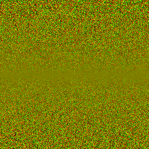
The Fourier amplitudes for negative K look very similar to the one for positive K, and once this step completes we get the final texture for the Fourier components for the z axis (the following gif shows how it changes over time):

Finally, the corresponding Fourier components for the x and y displacements (for 45º) will look like this:

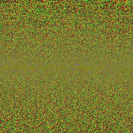
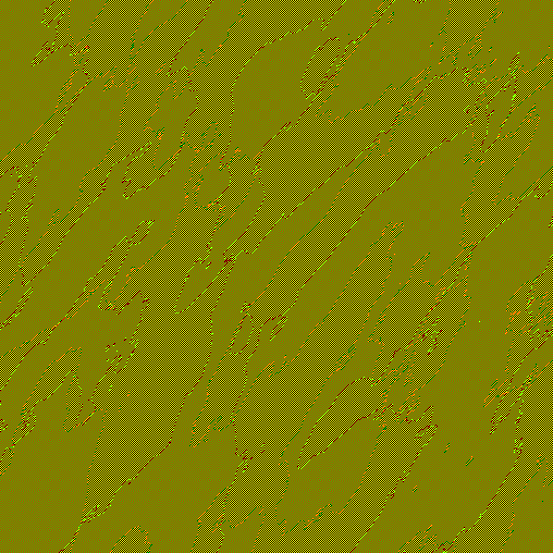
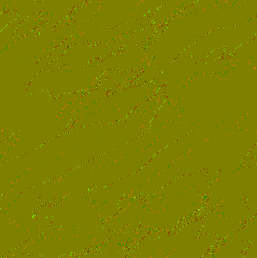
3. Performing the IFFT (Inverse FFT)

The IFFT is composed of 2 steps: performing N one-dimensional IFFTs across each row for each stage (log2(N) times), and then across each column. This is made possible to be done on the GPU thanks to the butterfly texture, which performs the row/column operations on the whole image at once for each stage. Note that there are some places where a divide-by-zero error can occur, and a single one can mess up the whole image (making result totally black in my case - from a single bad pixel!) - so this will need to be handled accordingly. Also note that GPU implementations often need to implement ping-ponging so that the output of one stage can be used for the input of the next. The following images show how the Fourier components for the x, y, and z displacements will be changed throughout each stage during the horizontal IFFTs:

Using the final stage of the horizontal IFFTs as inputs for the vertical IFFTs, we complete the operation with the following images as the result:

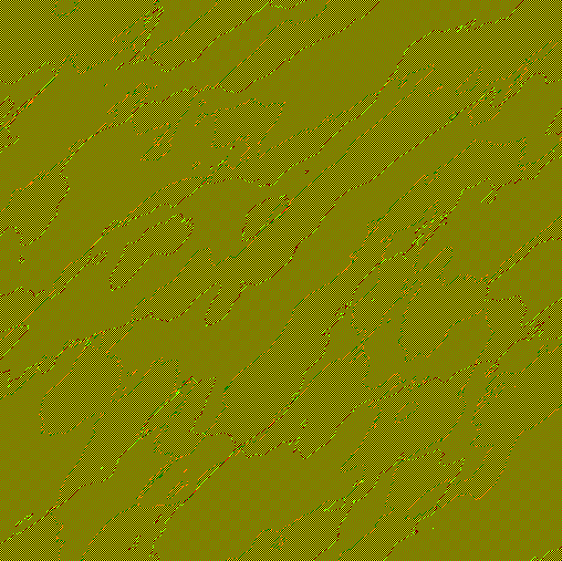
4. Obtaining the Final Displacement Map

The result of the IFFTs are not a jumbled mess of pixels anymore and look closer to ocean waves, but the values still need to be remapped to world space to create a displacement map (note that “displacement” refers to displacing the vertices of a flat plane with zero height, not displacing the heights from the previous frame). This is accomplished by applying a permutation and inversion operation to the result of the IFFTs (only the red channels are used) and creating a single texture from the 3 results, respectively storing the x, y, and z to the red, green, and blue channels:

Finally, the displacement needs to be mapped to world space. The x and y displacements are multiplied by the choppiness factor λ (usually -1) and, in my implementation in Unreal Engine, all three values are multiplied by 100 to convert the units in meters to centimeters (given that we have L=1000, the plane that this displacement would apply towards would be 100,000 centimeters long and wide). As such, we produce the following heightmap and its corresponding normal map (using Unreal Engine’s NormalFromHeightmap node, although this isn’t accurate as it only takes the vertical displacement into account - a better and more accurate way would be to generate a normal map from an IFFT as well):

Applying this heightmap to a tessellated flat plane in Unreal Engine, we can get the following animation:

5. Generating the Folding Map

This algorithm also provides a convenient way to identify where ocean foam and sea spray would occur on the surface of the waves. Considering that we are also displacing vertices by the x and y axes, sometimes they will get close together and even intersect - which happens in real-life, causing ocean foam and sea spray. This is called wave “folding”, and so the folding map masks all the waves that are steep enough to cause these effects. This is generated by using the determinant of the Jacobian matrix described in the linked papers above, which I get by using the following Material:

If the determinant is negative, then that means the waves are intersecting each other and thus “folding”. Modifying the various values of the simulation will produce animations like the following:

Finally, we get a foam texture and tile and mask it with the folding map, applying it to the ocean surface:

From a POV angle:

Modifications

As stated previously, the normal map needs to be fixed as it doesn’t account for the horizontal displacement. A potential solution could be to create a heightmap by sampling the displacement map according to the approach described in this video, thus producing a heightmap without horizontal displacement and generating the normal map from that.

Future Work

The next step is to implement particulate sea spray, which will be done using Niagara in Unreal Engine, and then shallow water dynamics by modifying this process to implement the iWave algorithm. Additionally,