Project: PlotEquation
Click to see gallery of full-sized images…
Introduction
It was my sophomore year in high school and it was my first engineering class I’ve ever taken. Mr. Niebergall, my engineering teacher, had mentioned to me that he is looking for a solution in bridging the gap between teaching engineering and teaching math, and that it would be a really nice addition to the CAD software Rhinoceros3D if it could generate math equations (much like Desmos) that students can then laser-cut and 3D-print. With my trigonometry-level math education (at the time) and a passion for programming, I discovered that making plugins in Rhino is really easy and well within my capabilities to provide a solution for my teacher. Within a week, I had a simple 2D cartesian equation grapher working (curves in the form y=f(x)), but I quickly realized that extending the plugin’s capabilities was really easy to do. By the next day, the plugin was able to graph 2D spherical equations as well (curves in the form r=f(Θ)), but this cracked open the door of opportunity even further as I realized extending these curves to 3D surfaces was really easy to do in Rhino. By the end of the next week, I had a fully functional 2D and 3D grapher (much like Geogebra) that could plot cartesian, spherical, cylindrical, and parametric curves and surfaces, and was able to 3D print my first mathematical object: a small 3D paraboloid. But I didn’t just print it out for fun: I wanted to see how strong it was and how much weight it could hold up. 473 pounds later I had run out of space to add any more weights from the weight room, and I realized the potential for this plugin was limitless. Flash forward 2 years later during my senior year of high school, and this plugin evolved to be much more than a simple equation grapher: it could now apply stereographic projections, generate various fractal objects, and more - far exceeding my engineering teacher’s original expectations. And thanks to this plugin, I was able to learn C# as well as gain a much more advanced understanding of mathematical concepts (such as quaternion algebra) well before I would be formally introduced to them.

Features
Surfaces
Cartesian Expressions: x=f(x,y); y=f(x,z); z=f(x,y)
Spherical Expressions: r=f(Θ,φ); Θ=f(r,φ); φ=f(r,Θ)
Cylindrical Expressions: r=f(Θ,z); Θ=f(r,z); z=f(r,Θ)
Parametric Expressions:
Cartesian: x=f(u,v), y=f(u,v), z=f(u,v)
Spherical: r=f(u,v), Θ=f(u,v), φ=f(u,v)
Cylindrical: r=f(u,v), Θ=f(u,v), z=f(u,v)
Implicit Expressions: 0 = f(x,y,z,r,Θ,φ)
Curves
Cartesian Expressions: x=f(y); y=f(x)
Polar Expressions: r=f(Θ); Θ=f(r)
Parametric Expressions (3D optional):
Cartesian: x=f(t), y=f(t), z=f(t)
Spherical: r=f(t), Θ=f(t), φ=f(t)
Cylindrical: r=f(t), Θ=f(t), z=f(t)
Implicit Expressions:
Cartesian: 0=f(x,y)
Polar: 0=f(r,Θ)
Miscellaneous
Stereographic Projections
Inverse Stereographic Projections
“4D” Expressions:
Cartesian: x=f(w,x,y); y=f(w,x,z); z=f(w,x,y)
Spherical: r=f(s,Θ,φ); Θ=f(s,r,φ); φ=f(s,r,Θ)
Cylindrical: r=f(s,Θ,z); Θ=f(s,r,z); z=f(s,r,Θ)
“4D” Parametric Expressions:
Cartesian: x=f(w,x,y); y=f(w,x,z); z=f(w,x,y)
Spherical: r=f(s,Θ,φ); Θ=f(s,r,φ); φ=f(s,r,Θ)
Cylindrical: r=f(s,Θ,z); Θ=f(s,r,z); z=f(s,r,Θ)
Fractals
Koch Objects:
Curve
Snowflake
3D Snowflake
Sierpinski Objects:
Triangle
N-gon
Pyramid
Tetrahedron
Octahedron
L-Systems: 2D and 3D
Mandelbrot Set: images, geometric objects
Evaluable Functions
• Sin(x)
• Cos(x)
• Tan(x)
• Asin(x)
• Acos(x)
• Atan(x)
• Round(x)
• Csc(x)
• Sec(x)
• Cot(x)
• Sinh(x)
• Cosh(x)
• Tanh(x)
• Random(x)
• Csch(x)
• Sech(x)
• Coth(x)
• Sinc(x)
• Sign(x)
• Exp(x)
• Pow(x, y)
• Log(x, y)
• Max(x, y)
• Min(x, y)
• RandInt(x, y)
• RandDec(x, y)
Gallery
See this post for a more expansive gallery regarding L-Systems.
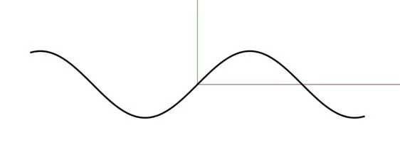
y = sin(x)

x = 4sin(t)^3
y = 3cos(t) - 1.3cos(2t) - 0.6cos(3t) - 0.2cos(4t)

r = Θ
Θ = cos(r)

Θ = 1/t, r = sin(t)

x = sin(πt)cos(t), y = sin(πt)sin(t), z = cos(πt)

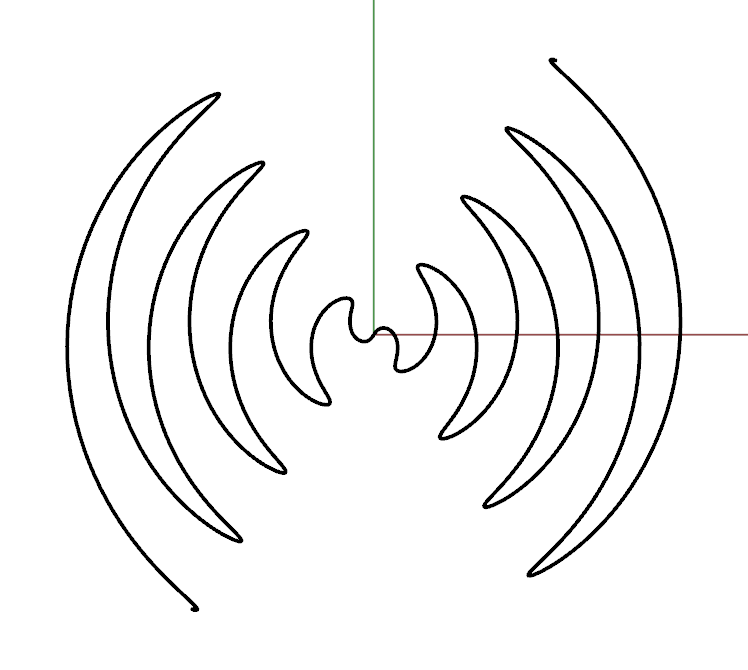
The Batman equation, before…

x = cos(t)^3, y = sin(t)^3

x = y^2

Θ = round(r, 0)

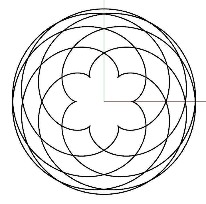
r = sin(4.5Θ)

Θ = sin(10t), r = sin(9t)

x = sin(πt)cos(t), y = sin(πt)sin(t), z = sin(πt)

… and after trimming the excess curves

Lasercut logarithmic spirals

z = x^2 + y^2

z = x^2 - y^2

r = cos(φ)^2

x = cos(v)^3 cos(u)^3, y = sin(u)^3
z = sin(v)^3 cos(u)^3

r = Θ


Gyroids that have been trimmed to a sphere

z = sin(w + x + y)

Transition between flat plane and cone

Flat design before…

… and after applying a stereographic projection

Classic Sierpinski Triangle

Inverted Sierpinski Triangle

Sierpinski Pentagon

Sierpinski Hexagon

Sierpinski Tetrahedron

Sierpinski Octahedron

Koch Snowflake

90-degree Koch Curve on a triangle

90-degree Koch Curve on a square

A 3D representation of the Koch Snowflake

Inverted 90-degree Koch Curve on a square

A 3D representation of the 82.15º Koch Curve

A skewed Sierpinski octahedron

The generated Mandelbrot Set…
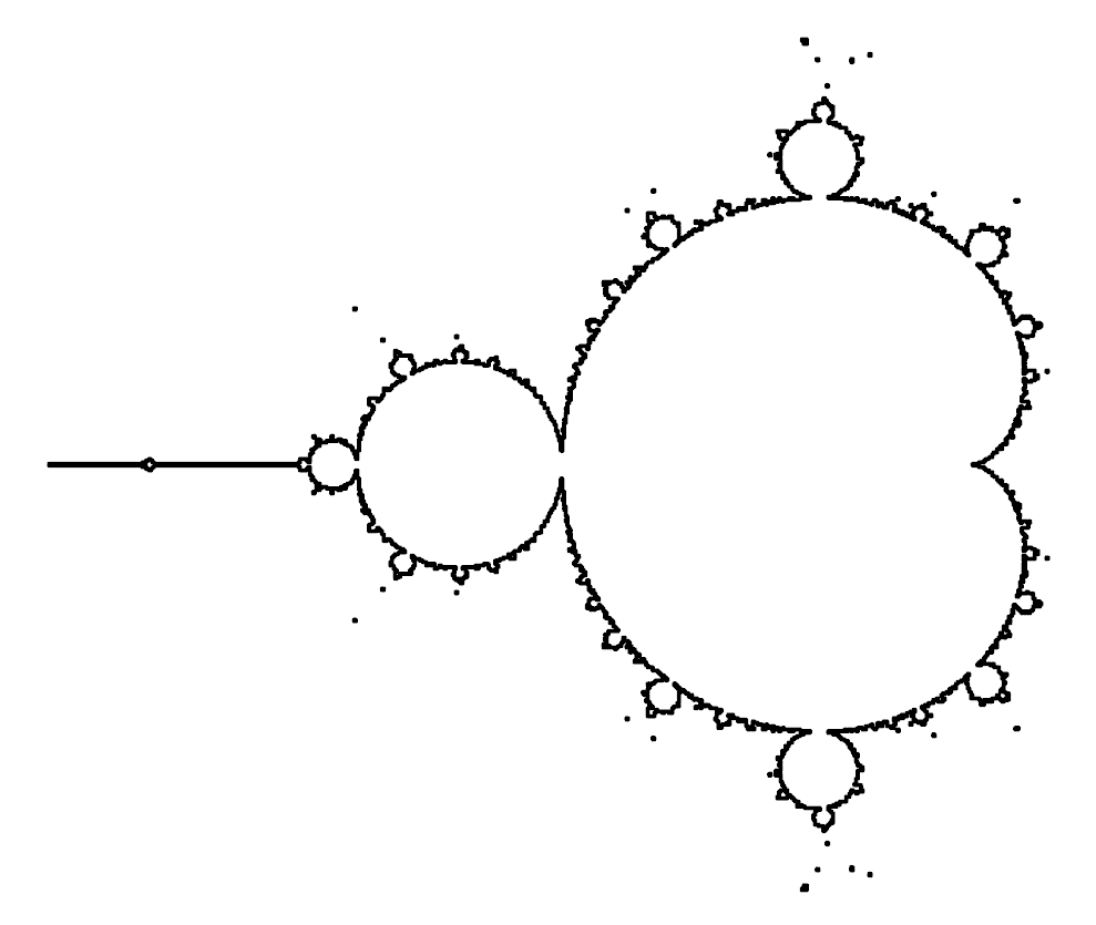
… which the plugin uses to create a set of curves

The Cantor Set, generated by the L-System A→ ABA, B→ BBB

A 90-degree Koch Curve, generated by the L-System F → F+F−F−F+F with a 90º turn angle
![The Pythagoras Tree, generated by the L-System A→B[+A]-A with a 45º turn angle, scaling each branch by half each iteration](https://images.squarespace-cdn.com/content/v1/601f19d09c6bdd6741ebb30f/1615122262312-PT3GN7LPHWW2Y0K8GSPR/pythagoras_tree-min-min.jpg)
The Pythagoras Tree, generated by the L-System A→B[+A]-A with a 45º turn angle, scaling each branch by half each iteration
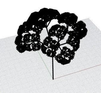
A 3D representation of the Pythagoras Tree, generated by an L-System

A 3D representation of the previous
L-System, with varying thicknesses
![An L-System generated by A→B[+A][A]-A with a 30º turn angle, scaling each branch by 2/3, 4/9, 2/3 each iteration, respectively](https://images.squarespace-cdn.com/content/v1/601f19d09c6bdd6741ebb30f/1615121455573-XG0SI0GHCP6HNZTKQYWW/tree_30_scaled-min.jpg)
An L-System generated by
A→B[+A][A]-A with a 30º turn angle, scaling each branch by 2/3, 4/9, 2/3 each iteration, respectively

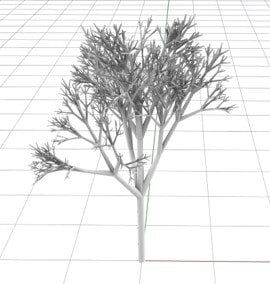
A 3D representation of the previous L-System

A 3D representation of the previous L-System, with varying thicknesses


.jpg)
3D representations of the previous L-System with random angles and thicknesses